Coming in as the thousandth time I've worked on rendering terrain comes Isle. At this point, though, I have come up on several useful techniques that I wanted to put together into a terrain generator with a bit more focus on realism. Relatively more realistic, that is, since the two prior projects, Planet Zoo and Country Terrains, both had very, er, optimistic colour palettes.
This post will go into detail on how to make interesting mountains with peaks and valleys, some methods for designing the colour palette, and effects to emphasise the map relief (contours, lights and shades).

Introducing Isle terrain. Here we see it in a dramatic aerial shot with perspective rendering. However, if I am to have any chance at explaining exactly what we are looking at and why it is interesting, I think it might be better to switch over to looking at maps.

This is not the same map, though the generator works the same. While the coastal outline of the Isle is the same as what you might expect from a simple noise algorithm, total altitude is a bit more complicated. Certain areas - picked by Perlin noise - are designated as mountainous. This is how we can find mountains with sharp declines down towards the sea, as well as have fertile lands with mild rolling hills in the middle of the island:
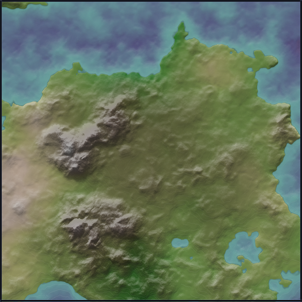
The method of designating mountainous areas is quite similar to what I described in depth in Greek Terrains. A Perlin noise field is used to designate areas as mountainous or not, independent of the basic terrain heightmap. Then this mountainnousness variable is combined with a high frequency third Perlin noise field for shaping peaks and valleys.

This totally fake 3D rendering goes a bit further in showing exactly what shapes the mountains take.
While the areas that are mointainnous is independent of the base height map, mountains are removed from underwater areas, which leaves the original island contour. This is done to avoid extensive reefs, and also creates interesting cliffs down towards the sea.
I'll describe the specific code for the peaks at the end of the post.
Since the generator was originally meant to render continents, that is, large scale terrain, the biome methodology described in Planet Zoo is also used here. A pretty simple Perlin noise field is put through a couple of transformations and then used to designate areas that are:

We can see an arid desert in the north-western corner, a jungle by the island to the north-east, and an intermediate, grassy green around the rest of the island.


Surprisingly, the very same terrain looks pretty neat in a 3D rendering. This really is the exact program, just in a different coordinate system. Oh, and then there's a sky with some cute clouds. The clouds however are not good enough to actually talk about at length. They are just a couple of Perlin noise fields multiplied with a third added in and a fourth one for shadows - but I just threw them randomly together until they looked nice.

This post will go into detail on how to make interesting mountains with peaks and valleys, some methods for designing the colour palette, and effects to emphasise the map relief (contours, lights and shades).
Introducing Isle terrain. Here we see it in a dramatic aerial shot with perspective rendering. However, if I am to have any chance at explaining exactly what we are looking at and why it is interesting, I think it might be better to switch over to looking at maps.
This is not the same map, though the generator works the same. While the coastal outline of the Isle is the same as what you might expect from a simple noise algorithm, total altitude is a bit more complicated. Certain areas - picked by Perlin noise - are designated as mountainous. This is how we can find mountains with sharp declines down towards the sea, as well as have fertile lands with mild rolling hills in the middle of the island:
The method of designating mountainous areas is quite similar to what I described in depth in Greek Terrains. A Perlin noise field is used to designate areas as mountainous or not, independent of the basic terrain heightmap. Then this mountainnousness variable is combined with a high frequency third Perlin noise field for shaping peaks and valleys.
This totally fake 3D rendering goes a bit further in showing exactly what shapes the mountains take.
While the areas that are mointainnous is independent of the base height map, mountains are removed from underwater areas, which leaves the original island contour. This is done to avoid extensive reefs, and also creates interesting cliffs down towards the sea.
I'll describe the specific code for the peaks at the end of the post.
- Arid
- Fertile
- Humid
We can see an arid desert in the north-western corner, a jungle by the island to the north-east, and an intermediate, grassy green around the rest of the island.
This means that colours are picked from two dimensions: Altitude and biome. Imagining the two to be linearly distributed along a rectangular spectrum, it would look like this:

Here we see the change from deep water to coastal shallows, to fertile terrain and into dark mountains and bright snow. At the top we see the light sandy colour of deserts, and at the bottom, the dark depths of jungles.
If this does not look like the pictures above, there are two reasons. First, obviously the terrain is not linearly distributed. Secondly, we are ignoring the altitude gradient and several effects applied to make it more obvious.
This is a blown up cut-out of terrain from the above map. It looks quite grainy, which is no mistake - the grain makes the terrain seem more realistic and physical, that is, when you do not zoom in to see the details.
The first effect is a bit straightforwad. An array keeps track of terrain heights, enabling quick comparisons when picking a pixel. Is the altitude higher than some of the pixels above it? The colour is made brighter to show off a north-south incline. Is it lower, showing a north-south decline? The colour is made darker instead. The change in brightness is related to the amount of change, but there is a roof which steep mountains almost always reach.
Related, but slightly different, you might notice some of the flatter areas also showing a north-south decline brightening, but rendered with random pixels instead of in a smooth blending. Here, comparison is only made to one pixel two spots above, and the change in brightness is constant - the treshold altitude difference is not, however.
The very same line of code also draws the contour lines, by taking the modulus of altitude of both this and the comparison pixel. If they both are within the same modulus range, the function works as above - but if the values cross over the modulus boundary, aka. contour line, the random limit is circumvented altogether.
And then a random pattern is made by blending the colour of the top pixel in each 2x2 area, just for added grainyness. I told you, I did this on purpose.
Surprisingly, the very same terrain looks pretty neat in a 3D rendering. This really is the exact program, just in a different coordinate system. Oh, and then there's a sky with some cute clouds. The clouds however are not good enough to actually talk about at length. They are just a couple of Perlin noise fields multiplied with a third added in and a fourth one for shadows - but I just threw them randomly together until they looked nice.
Finally, live demonstration and source code can be found at Openprocessing:
Perspective Isle
and
Map Isle
Mountain and peaks algorithm
I want to go into a bit more detail in how the mountains are shaped. It is a bit difficult, though. As it often happens, the final code came up through a lot of experimentation, and thus looks a bit odd. However, let us take a look at it.
//m denotes mountainousness
m = (noise(ix/250+1,iy/250+49)-.5)*.9
m = lerp(0,m,m*10)
h += m*(1+abs(noise(ix/50,iy/50+3)-.5))*max(0,min(1,-5+10*h))
I promise, if we clean it up a bit more, it's not so bad. The first line,
m = (noise(ix/250+1,iy/250+49)-.5)*.9
basically just sets up m to be a Perlin noise value:
m = (noise()-.5)*.9
Openprocessing returns noise values between 0 and 1, with an average of 0.5. This average is then subtracted, so that the distribution goes between -0.5 and +0.5, and then adjusted to be -0.45 to +0.45.
The next line actually stems from a typo, I believe, but the results were good enough that I kept it around. lerp() is linear interpolation, and interpolating a value from 0 and with itself - I believe that actually just squares m. How silly. Anyway, squaring the distribution creates more well-defined islands of high values (up to 2) and seas of low values (close to 0), as well as "folding" the negative parts of the distribution back into the positive. This explains the mountains passes running between two close-by mountain-ranges seen in some of the terrains.
Now, the third line is a bit of a doozy. Let us break it up a bit into the three values that are multiplied together:
h += m*mountainpeakheight*keepmountainsabovewater
We have already talked about m. Turning to mountainpeakheight, the full formula is:
mountainpeakheight = 1+abs(noise()-.5)
This outputs a value between 1, which is the lowest parts of the mountainous areas, that is, between the peaks, and 1.5, which is at the very top of a peak. Important to note is that we once again have a noise value subtracted by the average and then folded together.
Apparently this is enough to create those interesting peak shapes. Well, sort of. First off, the noise is pretty high-frequency. This means that one of the other effects, a coordinate offset, takes effect and shapes more fluid shapes. This offset is explained here and is one I basically use in all of my projects and often forget to think about.
Finally, the third factor:
keepmountainsabovewater = max(0,min(1,-5+10*h))
Keeps mountains above water. It is a bounded value between 0 and 1, which is 0 at sea-level and below, and 1 when fully inland. This removes mountains from underwater areas, as well as ensures that there are nice, smooth inclines down to the sea.
And I think that about does it.
Comments
Post a Comment