Last time, we went from the basics to a program that renders a chaotic composition. Today, we will add some more, important functions to the generation, and start to change the method of rendering.
This is what the results will look like at the end of this part:
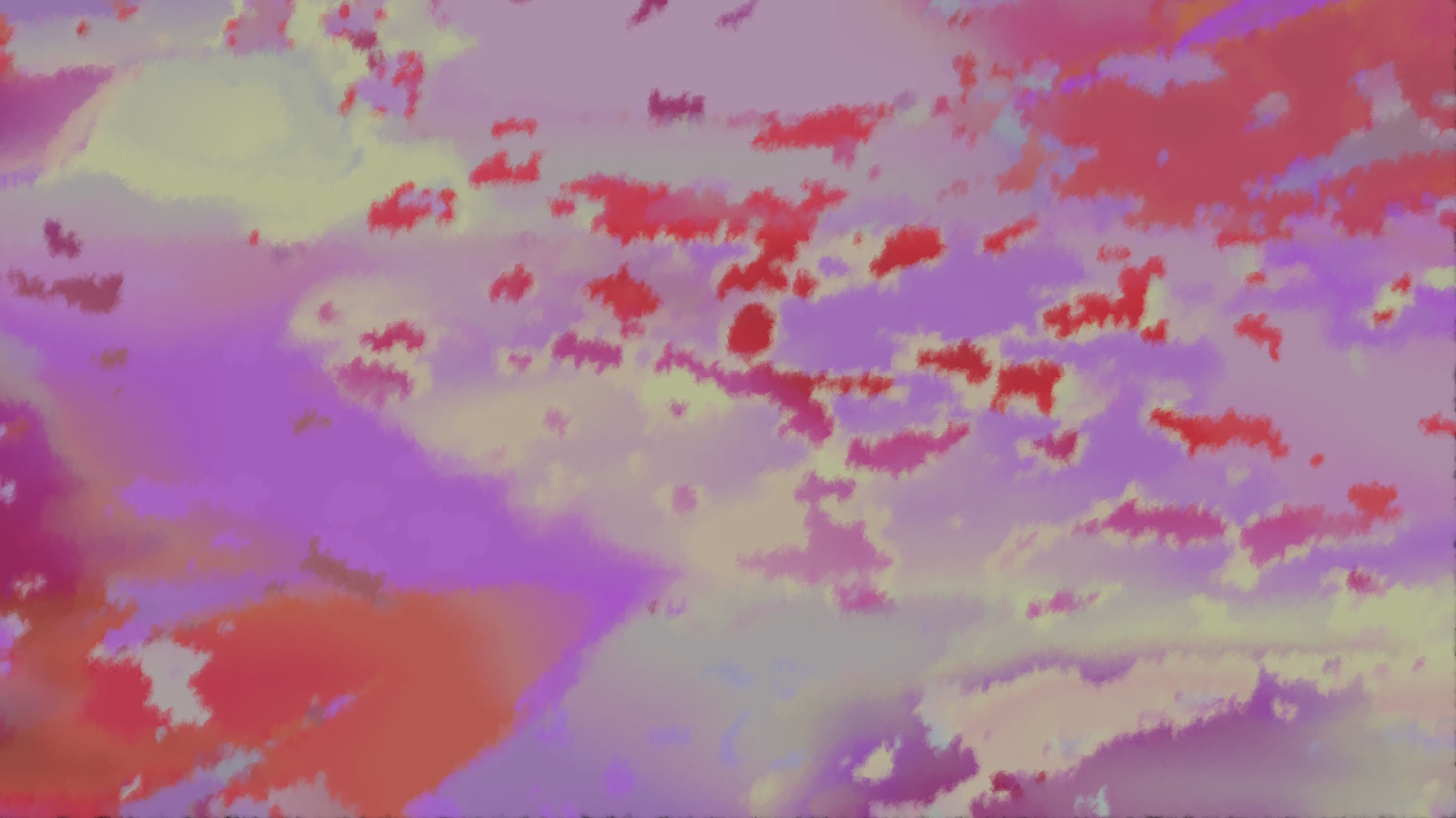
The code and the generator can be found at: https://www.openprocessing.org/sketch/581700.
So today, we will mature our generation process and turn renderings into paintings, or at least, lay the groundwork for it.
More functions
So far, we have three functions to combine previous neural layers, which all take in values in a 0-1 range and output values in a 0-1 range. This number can be expanded as much as we feel is necessary, but I will just add a couple more for now.
case 3: //using value C to interpolate between A and B
neuron[i+10] = lerp(inputA,inputB,inputC) ; break;
case 4: //taking the difference between A and B, offset by 0.5
neuron[i+10] = (inputA-inputB)/2+0.5 ; break;
case 5: //taking the distance between A and B, subtracted from 1
neuron[i+10] = 1-abs(inputA-inputB) ; break;
case 6: //find Perlin noise with coordinates offset by A and B
neuron[i+10] = noise((xcoord+inputA)*5,(ycoord+inputB)*5+10*i) ; break;
case 7: //same as above, but multiplying the noise by input C
neuron[i+10] = inputC*noise((xcoord+inputA)*5+10*i,(ycoord+inputB)*5) ; break;
The first new function works almost like the previous function, but instead of using a cutoff, it instead linearly interpolates between A and B. The next two functions are basically extensions of our previous, simple math functions, but here using subtraction instead of just addition and multiplication.
The last two functions, however, deal with Perlin noise. Here, the input values are used to offset the coordinates of the Perlin noise, meaning that the "terrain" of the Perlin noise will see sudden shifts when the values of the inputs change.
These are the single-dimension outputs of these functions when only looking at the 10th layer, that is, the very simplest:


Already here we see some more complex results.
Now, using all eight functions, our final neural layers look like:


If these look similar, it's because I still use the same random seed for the Perlin noise. Let me just go and change that, and then we can look at the kind of images that are now being composed:


Well, they certainly are more interesting than before. But there are still two apparent problems. One is that the colours are often quite flat, only ever blending between a few different pigments, not experimenting with shades and tints and such. The second is that things are getting overly crowded and not always in an all too pleasant fashion.
Let us first tackle the easier problem to solve - the colours.
Colour modification
Last time, we looked at two ways to make colours - by generating them through digital channels or by mixing different pigments. Above, I have opted for the pigment approach. But the best system is to use the pigment for the general colour, and then use the digital system slightly alter the resultant colour.
colAB = lerpColor(pigmentA,pigmentB,neuron[27])
colCD = lerpColor(pigmentC,pigmentD,neuron[28])
colABCD = lerpColor(colAB,colCD,neuron[29])
colred = red(colorABCD)+32-64*neuron[23]
colgreen = green(colorABCD)+32-64*neuron[23]
colblue = blue(colorABCD)+32-64*neuron[23]
fill(color(colred,colgreen,colblue))
As before, we first mix the pigments A, B, C and D into colABCD. But now, we split apart this colour into the three digital channels, red, green and blue. In each channel, we use a previously generated value to "nudge" the colour. Here, I multiply by 64, but depending on how you like your pictures different factor. If you want darker pictures, you might remove the +32, for instance.
Finally, the three colour channels are combined again to create the colour that we use to paint the screen. Let us see how this changes our renderings:


The colours have become more lively, perhaps more moody. At least to me, this is much more believable as art. But they still are not paintings.
The Shape of a Brush
function brush(nx,ny) {
maxradius = 15
beginShape(TRIANGLE_FAN)
vertex(nx,ny)
for(angle=0;angle<=PI*4;angle++)
{
length = maxradius*(.25+random(1.5)) ;
vertex(nx+length*cos(angle),ny+length*sin(angle)) ;
}
endShape()
}
This is what the results will look like at the end of this part:
The code and the generator can be found at: https://www.openprocessing.org/sketch/581700.
So today, we will mature our generation process and turn renderings into paintings, or at least, lay the groundwork for it.
More functions
So far, we have three functions to combine previous neural layers, which all take in values in a 0-1 range and output values in a 0-1 range. This number can be expanded as much as we feel is necessary, but I will just add a couple more for now.
case 3: //using value C to interpolate between A and B
neuron[i+10] = lerp(inputA,inputB,inputC) ; break;
case 4: //taking the difference between A and B, offset by 0.5
neuron[i+10] = (inputA-inputB)/2+0.5 ; break;
case 5: //taking the distance between A and B, subtracted from 1
neuron[i+10] = 1-abs(inputA-inputB) ; break;
case 6: //find Perlin noise with coordinates offset by A and B
neuron[i+10] = noise((xcoord+inputA)*5,(ycoord+inputB)*5+10*i) ; break;
case 7: //same as above, but multiplying the noise by input C
neuron[i+10] = inputC*noise((xcoord+inputA)*5+10*i,(ycoord+inputB)*5) ; break;
The last two functions, however, deal with Perlin noise. Here, the input values are used to offset the coordinates of the Perlin noise, meaning that the "terrain" of the Perlin noise will see sudden shifts when the values of the inputs change.
These are the single-dimension outputs of these functions when only looking at the 10th layer, that is, the very simplest:
Already here we see some more complex results.
Now, using all eight functions, our final neural layers look like:
Well, they certainly are more interesting than before. But there are still two apparent problems. One is that the colours are often quite flat, only ever blending between a few different pigments, not experimenting with shades and tints and such. The second is that things are getting overly crowded and not always in an all too pleasant fashion.
Let us first tackle the easier problem to solve - the colours.
Colour modification
Last time, we looked at two ways to make colours - by generating them through digital channels or by mixing different pigments. Above, I have opted for the pigment approach. But the best system is to use the pigment for the general colour, and then use the digital system slightly alter the resultant colour.
colAB = lerpColor(pigmentA,pigmentB,neuron[27])
colCD = lerpColor(pigmentC,pigmentD,neuron[28])
colABCD = lerpColor(colAB,colCD,neuron[29])
colred = red(colorABCD)+32-64*neuron[23]
colgreen = green(colorABCD)+32-64*neuron[23]
colblue = blue(colorABCD)+32-64*neuron[23]
fill(color(colred,colgreen,colblue))
Finally, the three colour channels are combined again to create the colour that we use to paint the screen. Let us see how this changes our renderings:
The colours have become more lively, perhaps more moody. At least to me, this is much more believable as art. But they still are not paintings.
The Shape of a Brush
Now, this part here is inspired by this post by the excellent Sighack, but I am going to go for a slightly simpler way to achieve a result mostly the same. If you want to expand on it, do go read their description.
Currently, we are drawing ellipses to render the colours onto the screen, but ellipses are boring, much too uniform. What we need is something with texture. This means it needs to have some randomness to it, it cannot be completely geometrically perfect. It has to have imperfections for the finished product to showcase a unique texture.
Again, here we might not be able to stay friends because different programming environments draw things onto the screen differently. The core idea, however, is simply to draw a fan of triangles in a very imprecise circle that loops over several times:
function brush(nx,ny) {
maxradius = 15
beginShape(TRIANGLE_FAN)
vertex(nx,ny)
for(angle=0;angle<=PI*4;angle++)
{
length = maxradius*(.25+random(1.5)) ;
vertex(nx+length*cos(angle),ny+length*sin(angle)) ;
}
endShape()
}
Specifically, it will look like this:
 But we really should not look for what it does like this, seperated, on its own. We should instead see what it does to our paintings:


In this broader picture, we can see the importance of using an irregular shape to render the picture, since it gives a natural texture to the painting. I would call it a feeling of a medium, instead of it feeling, as by default, plasticky.
Still, it's not perfect. All the brush strokes are identical in size and shape, and the paintings are, in essence, pointillist. But what we can do to change that is something we can look at next time.